CS 4641 Group 33: Predicting NFL Playoff Appearances

Introduction/Background

For our group project, we are trying to accurately predict whether or not a NFL team will make it into the playoffs based on their performance through the midway point of the regular season. In the NFL, there are 32 teams. Of those 32 teams, 14 teams will make the playoffs. There are two conferences in the NFL, the NFC and the AFC which each contain 16 teams. The conferences are further split into 4 divisions each (8 divisions total). The top team (based on record) in each division automatically make the playoffs. The division champions account for 8 out of the 14 teams that make the playoffs each year. The other 6 teams are wildcards. The three teams with the best record in each conference (after the teams that were division champions are removed) fill the remaining spots in the playoffs (3 teams from each conference fill the last 6 spots) [3]. The NFL regular season is 18 weeks long where each team plays 17 games because of one bye week. Another important aspect of the NFL is the NFL Draft. A teams order in the NFL Draft is determined by their previous season performance. The team who does the worst gets the first pick in each round, and the Super Bowl winner gets the last pick in each round [2].

Problem Statement

By creating a model that provides teams with a reasonable estimation on whether or not they will make it into the playoffs, we are providing actionable information. Teams need these predictions to make changes to their roster, budget, as well as decide whether or not to settle for a higher draft pick. For example, if a team uses this model to find out that they are most likely not making it into the playoffs, the administration can focus on trading players to better position the team for the following season. In regards to budgetting, this model could help teams prepare the stadium for Playoff season by allowing them to account for those preparations in their budget weeks in advance. Because of the structure setup by the NFL, teams do not get to keep the money from ticket sales during the playoff season. This means teams can actually lose money during the playoffs; therefore, a model that can predict if a team will need to account for an increase in spending after the regular season would benefit NFL teams immensely. Also, if a team is not predicted to make the playoffs by week 9, the team could spend less money picking up players in an attempt to save the current season. There is another benefit to knowing if your team will not make the playoffs: next seasons draft seeding. Intentionally throwing a season after using our model to learn the team won’t make the playoffs will cause that team to pick players ealier in the draft, enabling them to get the best talent coming into the league. We believe that by week 9 in the regular season, a machine learning model could predict with relative accuracy whether or not a team will make it into the playoffs that year.

Data Collection

For this project we manually retreived our data from multiple datasets on the Pro Football Reference Website [1]. Since the layout of the website requires the user to manually download each teams data for every season, we downloaded a csv file for each datapoint. Then, we used a python script to read and format the data into a final csv (NFLData.csv). This data contains one column for each feature and one column for our labels. The features we used were derived from the csv data files that we downloaded. We average the data from each team’s performance in the first 9 weeks of every season. These averages are saved in the data file along with a 1 or 0 in the label column. The 1 represents that team making the playoffs that season, and a 0 represents that team NOT making the playoffs that season.

All features used from this dataset are floating point numbers. When reading from the data csv’s coming from Pro Football Reference, we dropped data features like week (of the season), day of the week, and time of day as we do not think that these features would impact a team’s playoff possibility. We also dropped the feature focused on whether or not that game went into overtime. A problem we ran into while processing data from these sources was the possibility a bye week falling within the first 9 weeks of the regular season. This was represented by a row of Nan entries. In order to clean these entries from our dataset, we loop through each csv file and remove a row if there is a Nan present. In order to better understand our data, we first reduced the dimensionality of our data to 2D and graphed to view any major discrepencies or unexepected patterns/outliers. The graph of our model is shown below:

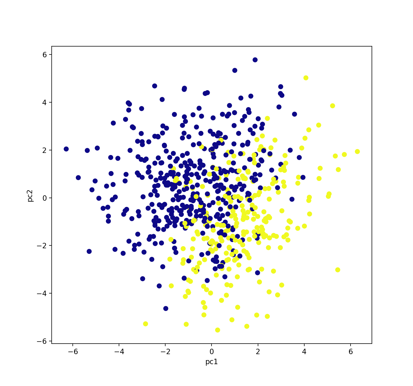
An interesting characteristic of our dataset is the number of datapoints labeled with 1’s vs the number of datapoints labeled with 0’s. Because our dataset covers the past three years of every NFL team’s season, there are more teams that do not make the playoffs (more 0’s) then there are teams that make the playoffs (1’s). This discrepency can affect the error in our model because our models could learn to classify every point as a 0 and still maintain an acceptable accuracy (above complete random 50/50).

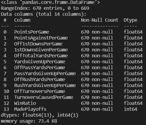
To address this problem, we realized that we need to get more data so that our model will be able to accurately classify points and not get trapped predicting all 0’s. We then adjusted our focus to adding to our dataset by creating a webscraping script that automatically pulls the necessary data off the Pro Football Reference website and formats that labeled data into a csv. This saved us a lot of manual labeling and pulling of data and allowed us to greatly expand our dataset. The total number of datapoints went from 96 to 670. The script that we wrote allowed us to get seasonal data for every team in the NFL for every season between 2000 and 2020. There was one team, the Houston Texans, that didn’t have data for 2000 or 2001, and this is because they did not have their NFL debut until 2002.

Once running our algorithms on the newly expanded dataset, we saw a pretty consistent accuracy, but it was lower than we were hoping, with the algorithiims averaging 75-80% accuracy. We took a closer look at the features we chose and the features available from the original dataset and decided that the win ratio is a valuable feature that could bring our models some higher accuracy. Because we had the script to web scrape all of this data and create a CSV file, we were able to quickly modify our features. The script takes roughly 2 minutes to get all of the data and create the CSV file, so adding the Win Ratio feature to our dataset was quite easy.

Methods

We downloaded CSV files from Pro Football Reference [1] and used a Python script to parse those CSV files, cleanse the data, and append it to the existing main dataset. We used Pandas to read the CSV into the dataframe and select the features from the dataset that we thought we most valuable to a team’s performance based on our football knowledge. The features we used were: Offense Average Points Scored, Defense Average Points Allowed, Offense Average First Downs, Defense Average Allowed First Downs, Offense Average Yards, Defense Average Allowed Yards, Offense Average Pass Yards, Defense Average Allowed Pass Yards, Offense Average Rush Yards, Defense Average Allowed Rush Yards, Offense Average Turnovers, Defense Average Turnovers, and Win Ratio. As stated above, these are all based on the first 9 games.

For this project, we used multiple different models to try to create the most accurate and consistent predictions. First, we used PCA to reduce dimensions and visualize our data. Next, we tried 4 different supervised learning algorithms: Ridge Regression, Logistic Regression, Neural Network, and Support Vector Machine. We had to normalize our data before plugging it in to these models because the features were on different scales. (For example: One of our features, passing yards, is usually in the hundreds, whereas another feature, turnovers, is usually less than 7). Logistic Regression, Support Vector Machine and Ridge Regression all use the sklearn library. For the neural network, we used the keras library. We ran logistic regression and the neural network on the dataset that had been dimensionally reduced by PCA, and also on a dataset that had all of its dimensions. This provided valuable information to see if we are overfitting when we include all of the features.

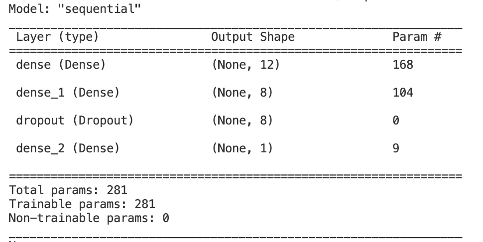
The Ridge Regression model uses an alpha value of 0.01 and runs for 3,000 iterations. This model is an attempt to fit the training data with a line. We chose ridge regression to add in some bias to our model so that we do not overfit the training data as we do not have a very large dataset. For the Logistic Regression model, we use the LogisticRegression class from sklearn’s linear_model. We train this model for 10,000 iterations. The support vector machine is implemented using the svm class from sklearn. This model attempts to separate the data with a decision hyperplane. This implementation uses the rbf kernel in order to better fit the potentially non-linearly separable dataset that we passed into it. Finally, we created a neural network model using keras. This model uses 2 fully connected layers with relu activation functions as well as l2 kernel regularization in each layer. Then, we have an output layer with one node and a sigmoid activation function to make the classification for this problem. We use batch gradient descent with a batch size of 10. The neural network description is found below.

Neural Network Description:

Results

Logistic Regression without PCA performs well for our model with a best-case accuracy of 0.887. Logistic Regression with PCA has a slightly lower accuracy with a best case of 0.863. The neural network trained on the reduced dimmension dataset has a best case accuracy of 0.815 on the test set. The accuracies vary slightly because we do not have static training and testing data sets. We randomize which part of our dataset is testing and which part is training each time we run the algorithm, which helps us see how robust our model is and if we are overfitting.

Best-Case Logistic Regression with PCA:

Test Set Accuracy = 86.3%

Best-Case Logistic Regression without PCA:

Test Set Accuracy = 88.7%

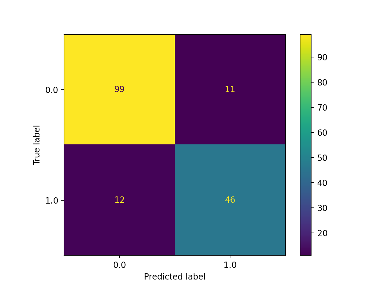
Best-Case Neural Network with PCA:

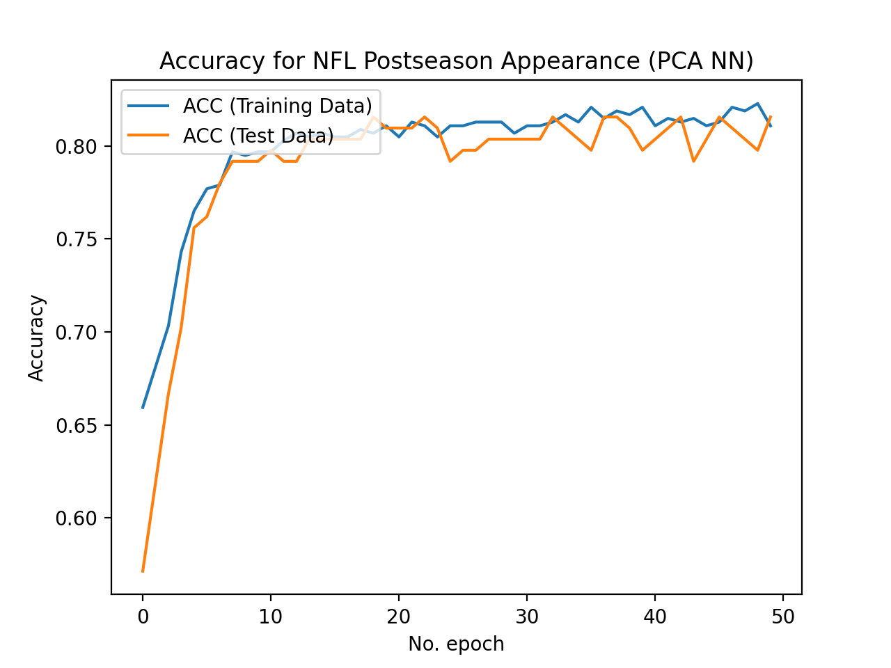Test Set Accuracy = 81.48%

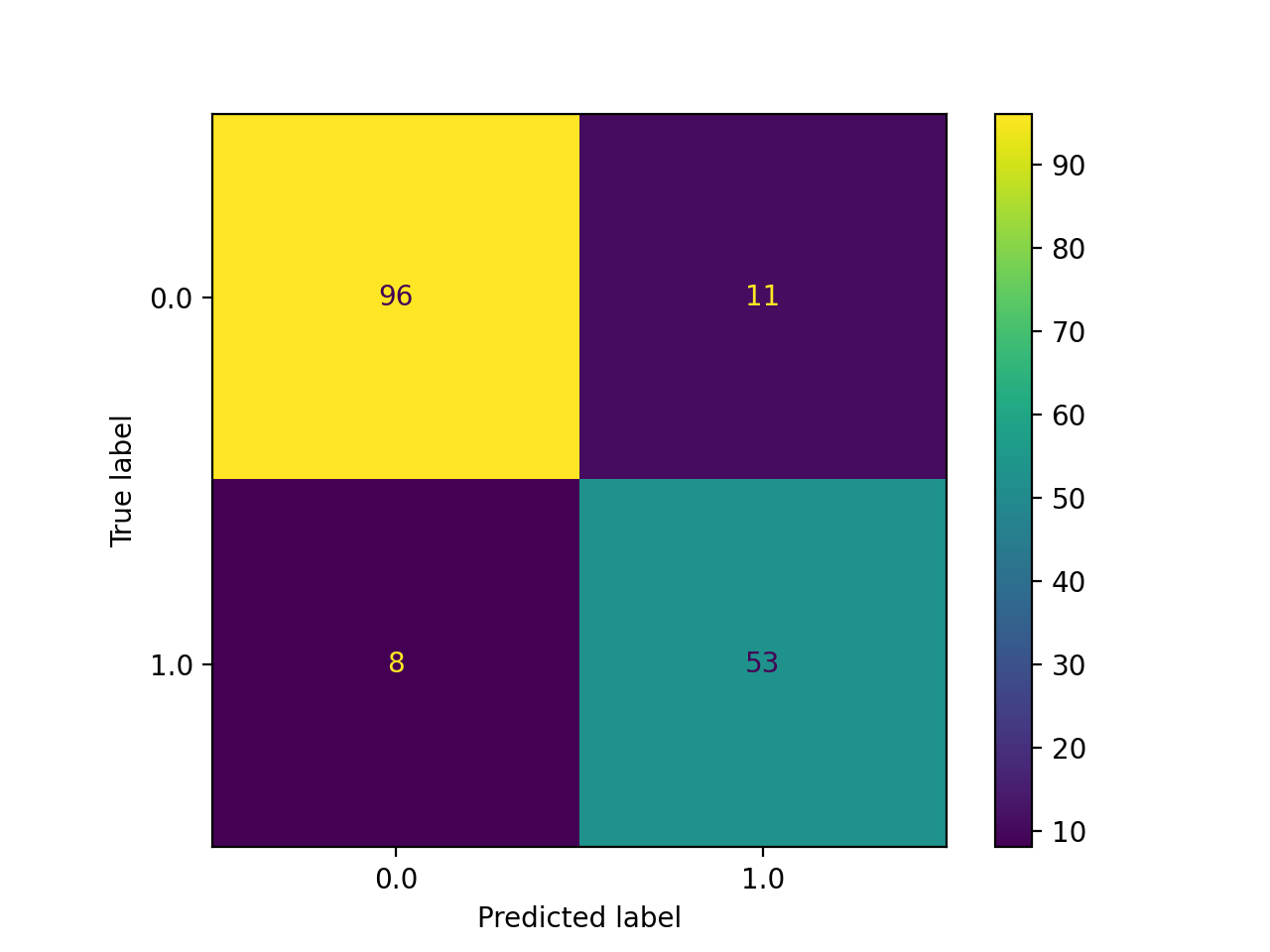
Best-Case Neural Network without PCA:

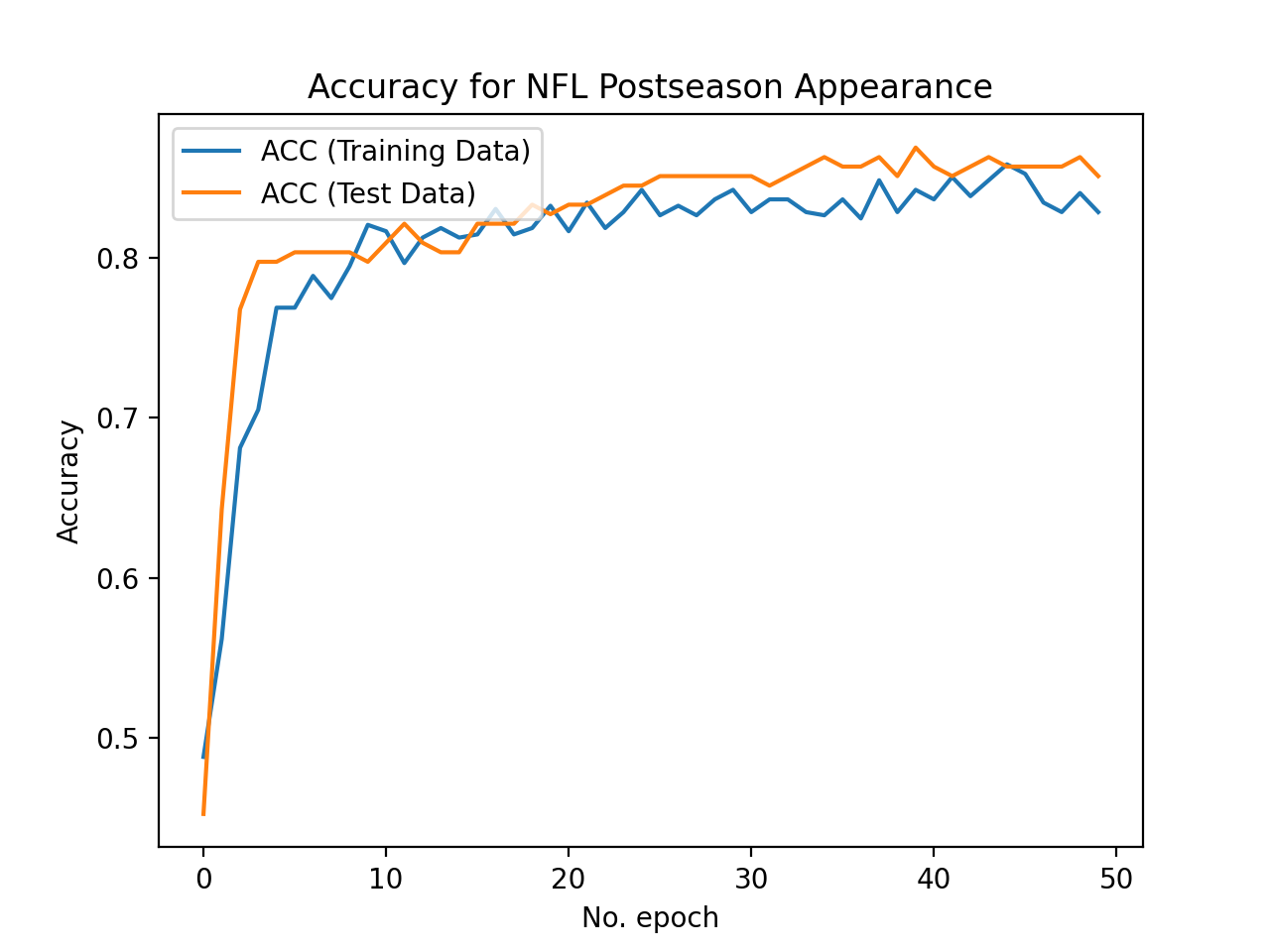Test Set Accuracy = 85.03%

Worst-Case Neural Network without PCA:

Test Set Accuracy = 79.8%

Best-Case Support Vector Machine:

Test Set Accuracy = 88.69%

Comparing Accuracy of Algorithms:

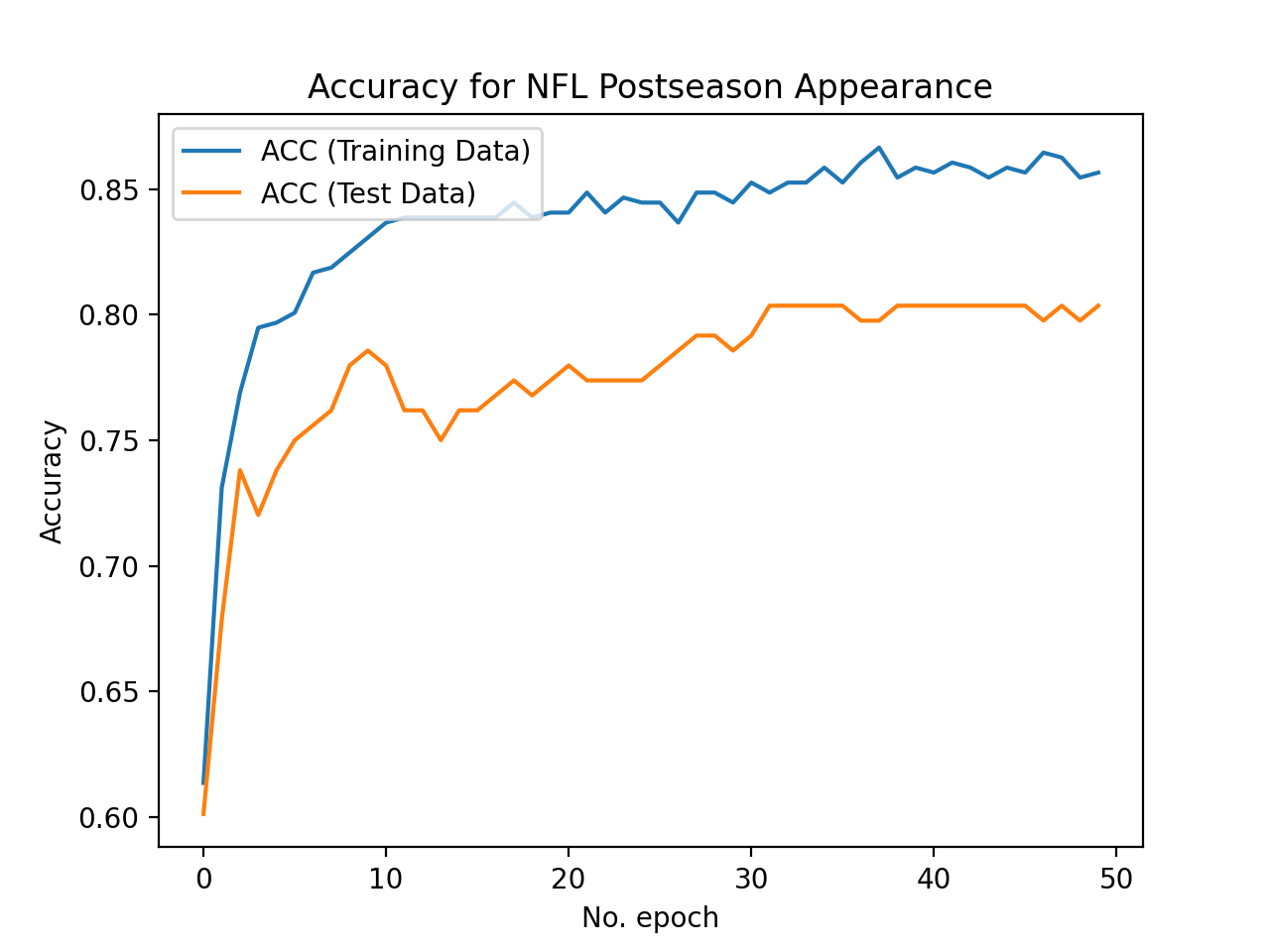
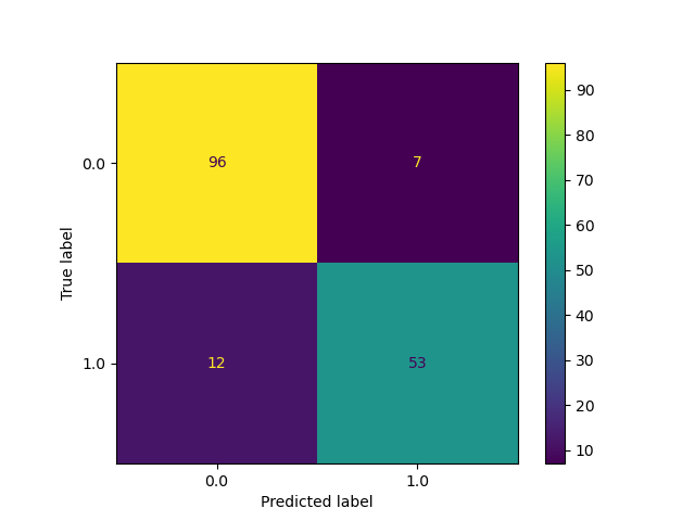
We use the train_test_split method within sklearn’s model_selection class to create our training and test sets from our data. We make 75% of our data set into training data points and the other 25% is used for testing (validation). We commonly use the ConfusionMatrix method within sklearn’s metrics class to visualize how each model is classifying on our test (validation) set. This matrix allows us to easily visualize the false positives and false negatives in the model and helps us to understand if we are overfitting or underfitting. We also use plots of accuracy on the test set by number of iterations to decide on the appropriate number of iterations for each model to converge. These plots also help us visualize overfitting because we plot the curve for the training set accuracy as well as the test set accuracy. If the training set accuracy is very high but the test set accuracy remains low on the plot, then it is clear that we have overfit the data and need to either get more data or add regularization. In the ‘Worst-Case Neural Network Without PCA’ this trend is clearly shown as their is a gap in accuracy between the training and test set. To address this, we added a dropout layer to the neural network with a rate of 0.30. This regularization helped the test and training data performance converge to a higher average accuracy of around 0.83. There is still room for our models to improve, but we believe that we have tuned our models to their maximum potential given the dataset and features used.

Discussion

In order to improve our models (target accuracy of 95%), we believe that we need more data. We have written a python script to scrape data from the website which has increased the size of our dataset greatly; however, we still do not have enough data to train a very large model that can fit the intracacies of this complicated problem well. For example, our neural network is only 4 layers with only 281 trainable parameters. When we made learning curves of networks with more trainable parameters, the overfitting got worse in our model. We added a dropout layer to our network to help us address the overfitting, but we were not able to generalize enough using regualrization to train a large fully-connected network on only 502 training datapoints.

As shown in the results, performing PCA to reduce the dimensionality of our dataset before training a logistic regression model and neural network did not improve the accuracy. Principal Component Analysis enabled us to visualize the data which was helpful for understanding the grouping of our data in two dimensions. When the dimmensionality of the data was reduced, we most likely lost some information that related to the output of making the playoffs; therefore, it is understandable that the models performed worse when trained on the dimension-reduced data set.

It makes sense why PCA does not really work, as if you think about it, there is no “clear cut” way for a team to win a game of football. Some teams don’t have a very strong offense, but their defense makes up for it, letting the team pull out a win. This would mean that the defensive features would have high importance for those teams making the playoffs. Other teams have horrible defenses with dominant offenses, giving an opposite image of feature importance. Therefore, when PCA is run, it changed the number of dimensions from 12 to 2, definitely removing some features that are not very important to the majority of the training set, but are still important to a lot of other datapoints, resulting in low test accuracy.

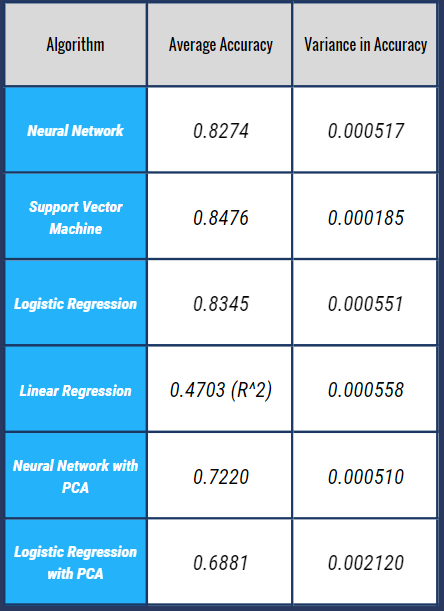
The Support Vector Machine algorithm consistently performs the best on our dataset. We used learning curves to tune the hyperparamter C in order to maximize the accuracy on the test set for this model. As C increases in size, the model forms a smaller margin. We plotted C values ranging from 0.0001 to 100 to find which range created the best model for our data set. Based on our learning curves, we concluded that the SVM model performs best when C = 0.5. In addition to having the highest accuracy, SVM also has the lowest variance on our dataset. Therefore, SVM with an rbf kernel appears to be the best algorithm for fitting our problem given our dataset.

The next highest performance was logistic regression; however, both the logistic regression model and the neural network performed very similarly. Logistic regression had an average accuracy that was 0.7% higher than the neural network but also had a higher variance (0.000034 higher). The logistic regression model works well for this problem because it is a binary classification problem where our features are continuous variables. The neural network performs well because of the number of parameters that it trains. The model can fit complex trends in data because it trains a high number of parameters being a fully connected model. The limiting factor on our neural network performance is the size of the dataset. Because we only have 502 training datapoints, our neural network cannot adequately generalize when we train a large model with thousands of trainable parameters.

The worst performing model in our set was linear regression with an average R^2 value of 0.4703. A high performing ridge regression model achieves an R^2 value near 1. We believe that ridge regression does not fit our dataset well because of the extremely non-linear nature of the problem. SVM solves this by using a kernel and soft margin (which tolerates misclassifications), but linear regression struggles to fit the non-linear, complicated dataset.

Conclusion

Hoping to predict NFL teams’ playoff placement given their first 9 games, we web scraped NFL data from the past 20 years, cleansed the data, and put it through six different algorithms: Neural Network, Logistic Regression, Linear/Ridge Regression, Support Vector Machine, Neural Network with PCA, and Logistic Regression with PCA. Once increasing our dataset we saw an overall decrease in accuracy, which did not surprise us. In an attempt to increase our accuracy, we added a Win Ratio feature to the dataset, which worked well, increasing our accuracy by 5-10%. Before expanding our dataset, Logistic Regression without PCA gave us the best accuracy, averaging just below 80%. Once expanding our dataset, Support Vector Machine consistently gave us high accuracies, with an average accuracy just below 85%. Since we have a relatively small dataset with only 670 datapoints, we used a Neural Network architecture that was more suited for smaller datasets. We realized that the curve flattened pretty quickly so only 50 epochs were needed. Although we are very happy with the accuracies we are getting, we have realized some of the difficulties of predicting NFL playoff placement. One thing that is hard to account for is the fact that there is no one team composition that will get an NFL team to the playoffs. This complicates Machine Learning algorithms, as features do not have uniform importance for each team’s playoff chances. Thankfully, our models still performed quite well and have the potential to produce valuable information.

References

[1] https://www.pro-football-reference.com/
[2] https://www.sportingnews.com/us/nfl/news/how-does-the-nfl-draft-work-rules-rounds-eligibility-and-more/o431yshp0l431e7543pcrzpg1
[3] https://www.si.com/nfl/2021/01/09/nfl-expanded-playoffs-explained

PS: Who is Making the Playoffs This Year?

New England Patriots, Buffalo Bills, Tennessee Titans, Baltimore Ravens, Cleveland Browns, Denver Broncos, Dallas Cowboys, Tampa Bay Bucaneers, Carolina Panthers, New Orleans Saints, Green Bay Packers, Arizona Cardinals, and the Los Angeles Rams. These predictions were made using our SVM model.